Excel for iPad: Top 11 tips
Juggle your spreadsheets on the iPad with our guide to the Excel app

It's been two years since Microsoft launched Excel for iPad, and while it may have seemed like a slightly foolhardy move at the time, Apple's tablets have proved themselves to be more than capable of handling complex spreadsheet manipulation. Despite lacking a full keyboard and mouse interface, Excel for iPad is very nearly the equal of its desktop counterpart.
Here are our top 11 tips to get the best our of Excel on your Apple tablet.
1. Work on more cells at once with the iPad Pro
Apple's mammoth 12.9in tablet has been touted for its use as an enterprise prodcutivity tool, and so it's no surprise that Microsoft has brought out a special version of its app to take advantage of the iPad Pro's larger screen.
In addition to a larger screen surface to work across, the addition of the Apple Pencil and Smart Keyboard means that users can have much more delicate control of their spreadsheets, without worrying about deleting something vital with one ham-fisted swipe.

However, users should be aware that after the first 30 days, you'll need an Office 365 supscription to do anything more than view spreadsheets with the iPad Pro.
2. Duplicate before doing anything complex
Excel for iPad can be too powerful for its own good. If you're working on a spreadsheet created on a PC/Mac that has tons of formulae, pivot tables or other complex formatting, it's possible to accidentally clear the contents of a critical cell or drag a table out of place as you're swiping around the document.
The undo button in the top left corner can come to your rescue if you notice your mistake, but it's easy to damage something without noticing, and because the app is set to autosave by default.
Get the ITPro daily newsletter
Sign up today and you will receive a free copy of our Future Focus 2025 report - the leading guidance on AI, cybersecurity and other IT challenges as per 700+ senior executives
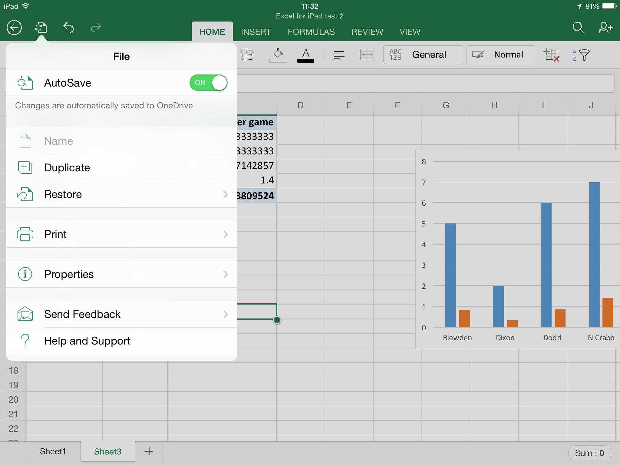
If you're planning to work on a complex spreadsheet on the iPad, it's best to click the Save menu button (the little page icon with the two arrows) and click Duplicate before you get going. Then if you make any mistakes, you've got the original to fall back on, without having to rely on the Restore function.
Autofill is one of the most useful features of Excel on the desktop. It spares you from laborious entry of text or formulae by second guessing what you want to appear in the column or row. So, for example, if you've got a spreadsheet analysing daily sales figures, you might have the days of the week running down a column. With Autofill you can type "Monday" and "Tuesday" in successive cells, and then drag down to Autofill the next five cells with the remaining days of the week.
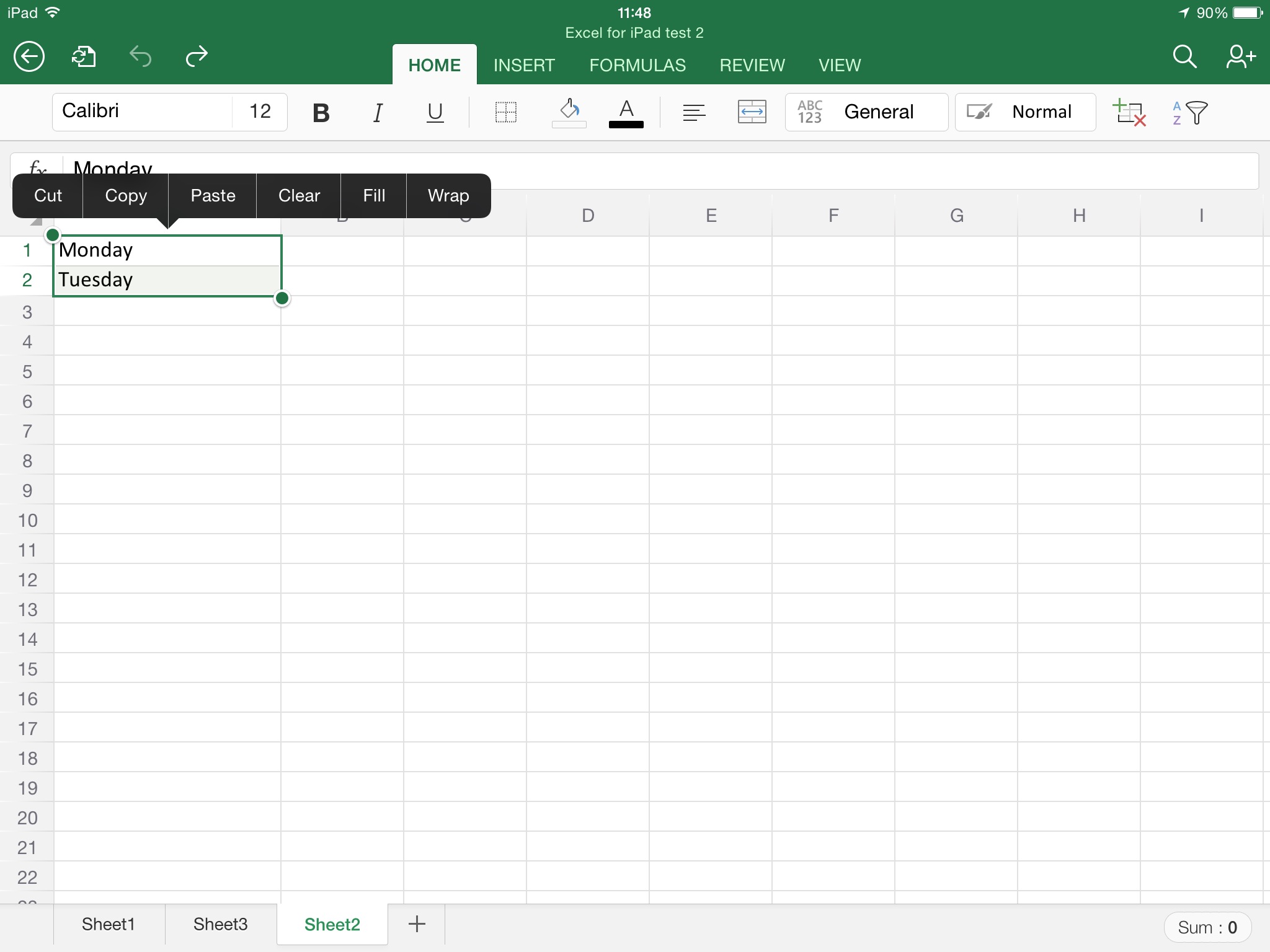
In the desktop version of Excel, Autofill is activated by clicking on the bottom-right corner of a selected cell and dragging downward/sideways. On the iPad, you first need to select the cells in question, by clicking on the first cell and then dragging the little circular handles down to the last. Then a pop-up menu will appear, with Fill among the options. Click that and drag the arrows that appear on your selection either downwards or sideways to Autofill the contents.
4. Moving the contents of rows or columns
Sometimes you might find you want to move the contents of an entire row or column to a new location. Trying to manually select all the data in a long row or column might be awkward on an iPad, but there's a much easier way to do it.
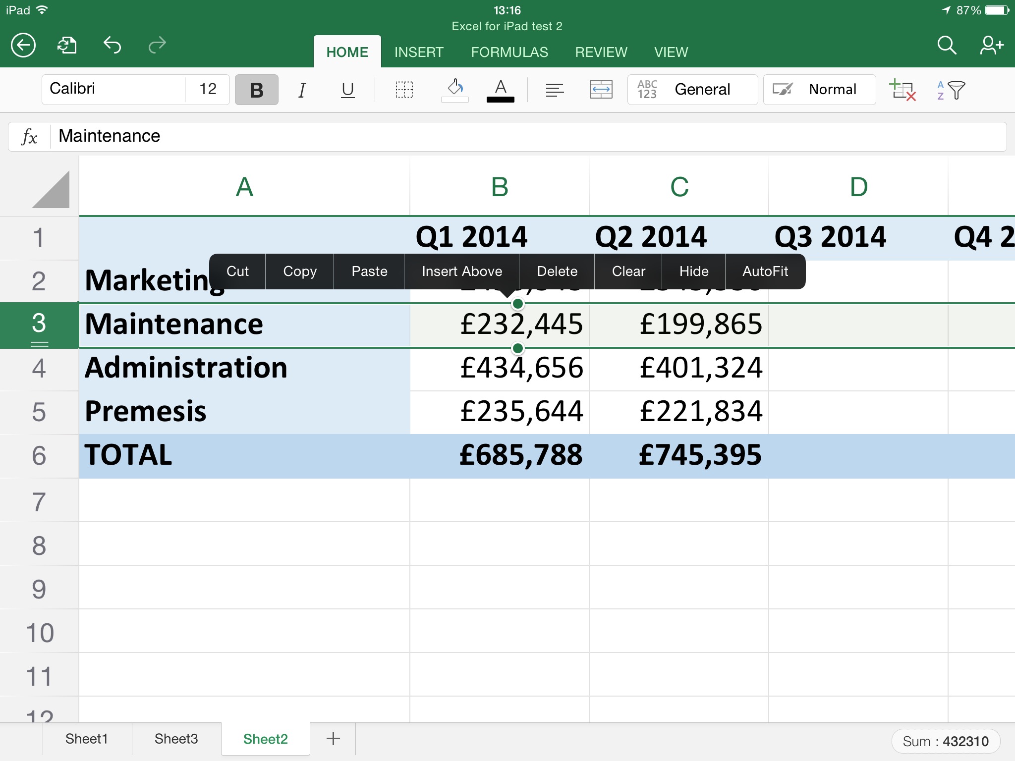
Click on the column/row's number or letter and the entire column/row will be highlighted. A pop-up menu will appear: select Cut. Now tap on the column to the right of, or the row below, where you want to paste the data and press Insert Left or Insert Above. The data will be pasted into the space, with the other columns/rows automatically shifted so that you don't leave an empty space in the worksheet.
5. Easy Autofit
If you find the content of cells is not fully displayed because the column width or row depth isn't sufficient, there's a quick way to solve this: double tap on the column/row's number or letter and the contents will Autofit so that you can read them fully.
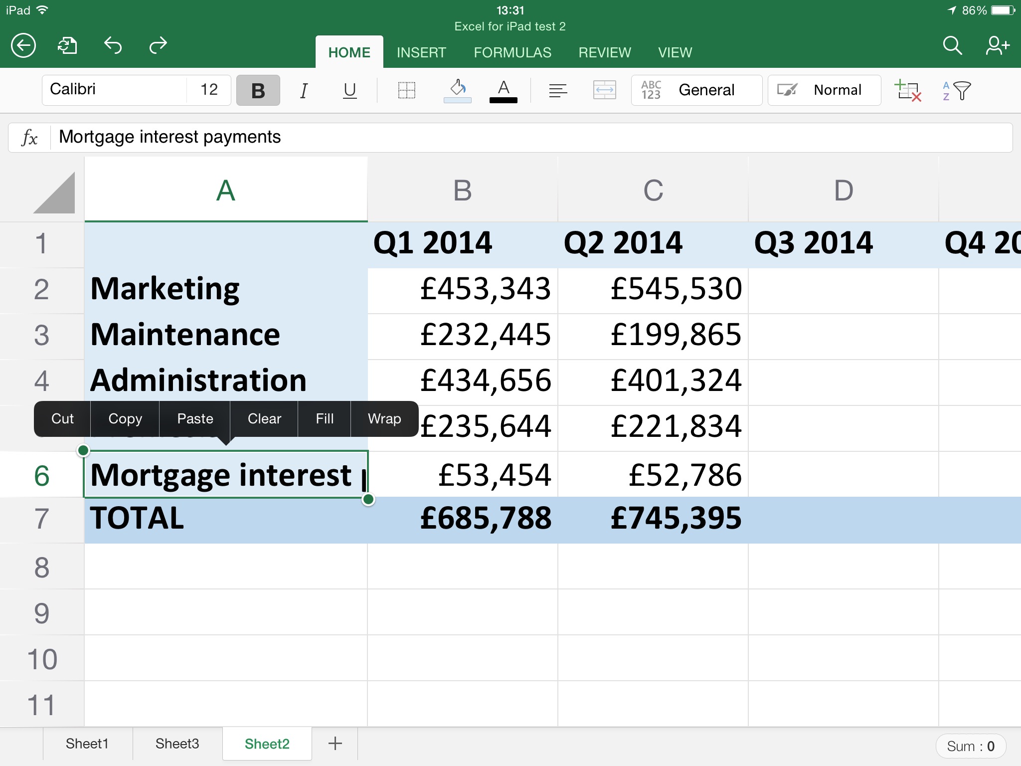
If the content of only one cell in a particular row or column is running out of its box, it might be neater to simply wrap the content of that cell, rather than make the whole column/row bigger. To do so, tap on the cell to select it, and then tap again after a short pause (i.e. don't double tap) to bring up the Edit menu, and then select Wrap.
6. Combining selected data
Let's say, in the table shown in the screenshot below, that you wanted to create a separate row beneath the main table showing only the building costs (i.e. Premises + Mortgage Interest Payments) for each quarter. There's a simple way of doing it without writing the formula by hand.
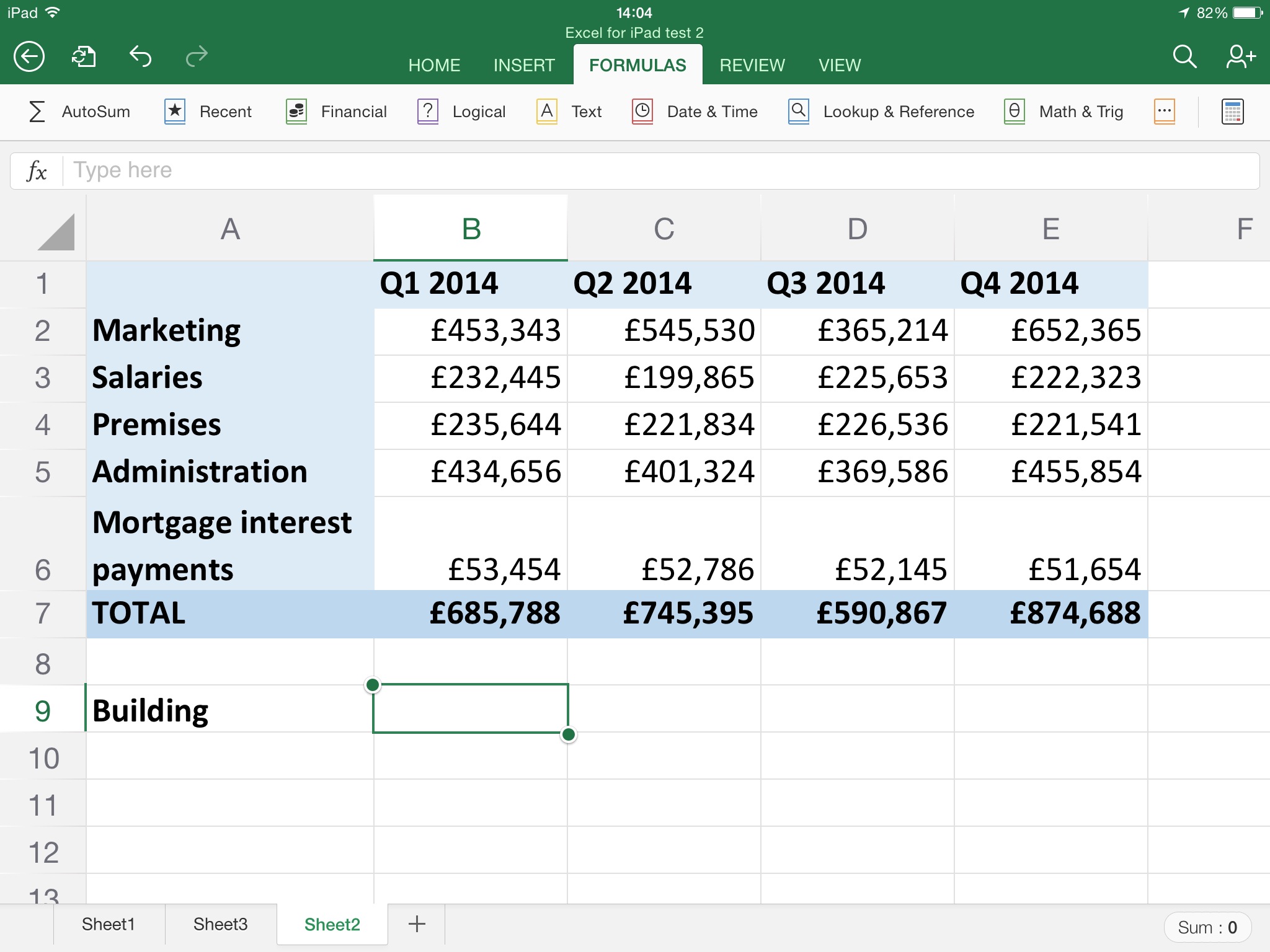
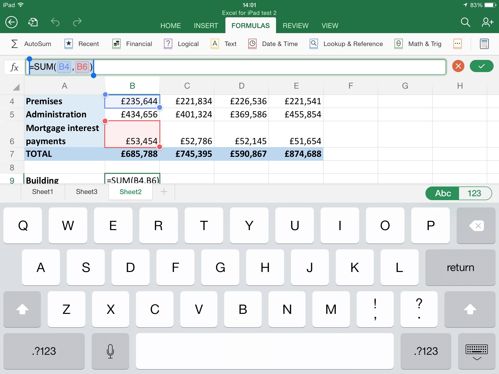
Select the cell you wish to use (in our case B9), go to the Formulas tab and select Autosum and choose the SUM formula. Excel will assume you want the total for the entire column, which is incorrect. Instead, just tap on the cell B4 (for Q1 Premises costs) then type a comma, and then select the cell B6 for Q1 mortgage payments, and click tick to apply. You can, of course, use the Autofill technique from Tip 2 to apply that same formula for building costs across every quarter.
Barry Collins is an experienced IT journalist who specialises in Windows, Mac, broadband and more. He's a former editor of PC Pro magazine, and has contributed to many national newspapers, magazines and websites in a career that has spanned over 20 years. You may have seen Barry as a tech pundit on television and radio, including BBC Newsnight, the Chris Evans Show and ITN News at Ten.